Data Science CS109 Final Project - Fall 2014
Ahmed Hosny, Jili Huang, Yingyi Wang
The Green Canvas: Art Valuation Analytics from yingyi on Vimeo.
Background and Motivation
The team is interested in quantifying aesthetics as an extremely subjective and quality-based feature. We are all from design background and we always want to explore the middle realm between artistic evaluation and scientific statistics. How to evaluate a painting? Will there be any interesting relationships between its evaluation (in terms of price) and its pixels? Taking into consideration other factors such as artist's prominence, the project will attempt to answer questions such as: Are paintings of specific contrast tend to be evaluated higher than those with high saturation? Are paintings with sharp edges or on bigger canvases tend to sell cheaper? Focus will be on contemporary paintings as a twist on the exaggerated prices some of these pieces have reached - especially when many are comparable to children's artwork.
Project Objectives
This project aims at studying art valuation criterion with a specific focus on paintings. While the art market itself is responsible for fluctuations and trends, aesthetics plays an important role in evaluating art pieces. Image processing will be utilized to extract pixel information and attempt to correlate these with the peices' current market value. Therefore, the plan is to:
- Use data to explore trends in painting evaluation. How is information about the painting or even at the pixel level influencing evaluation?
- Develop a machine learning framework that can predict pricing. Can we develop an algorithm that can replace expert art consultants and can be used by, say, auction houses?
Data Acquisition
Data will be collected from two sources:
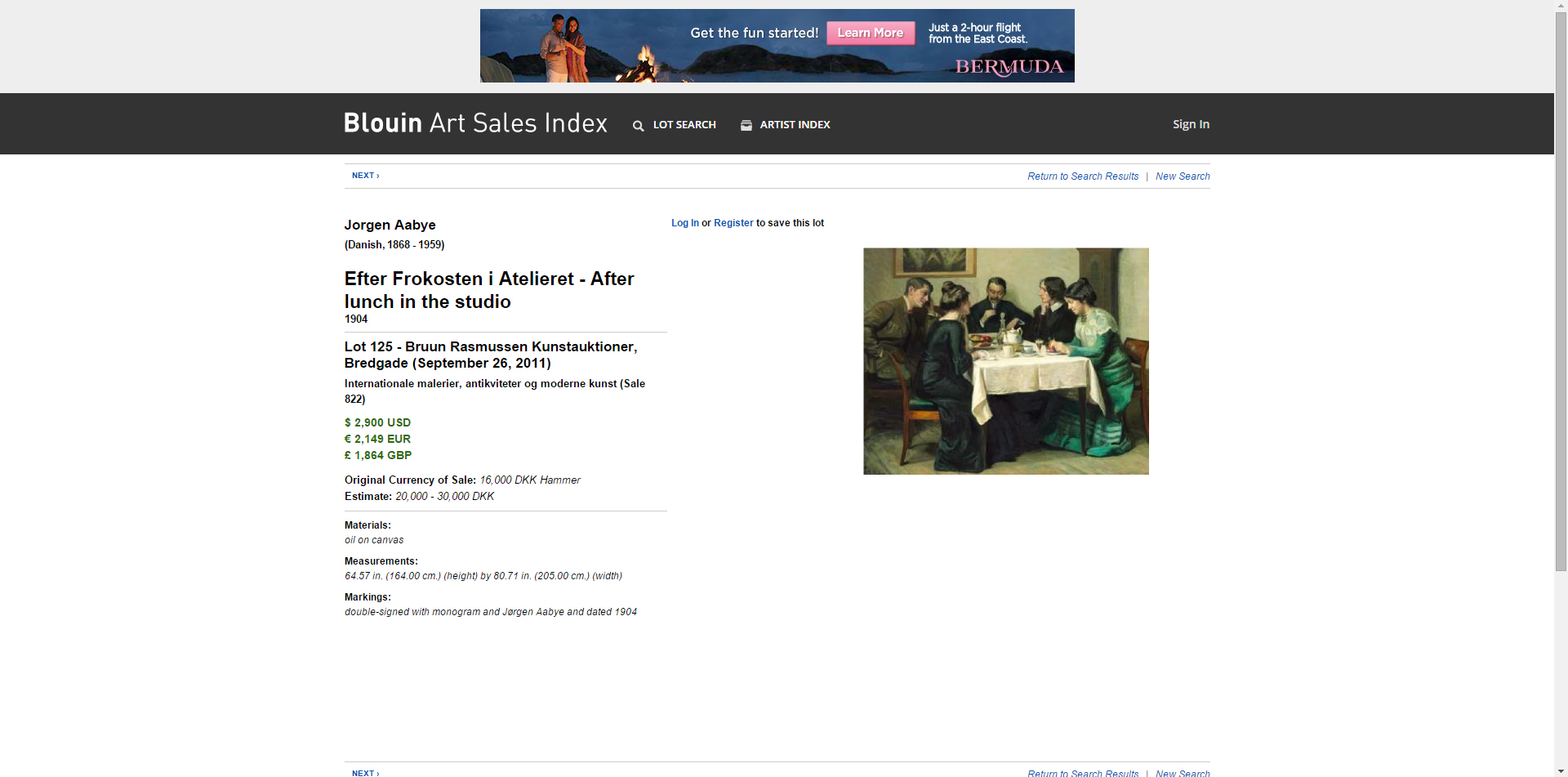
- Internet: Scrape information off websites such as http://artsalesindex.artinfo.com/asi/lots/3426445 . A Pandas dataframe will be constructed containing the columns: Artist's name, Year, Country, Painting Name, Style, Material, size, Markings and Price with time sold.
- Image of the painting itself: Use openCV and PIL libraries to add features to the dataframe such as: Face detection - tell us whether it is a portrait or not, Top dominant colors, large/small Areas of solid color, Edges, contrast, brightness, hue, saturation…
Design Overview
This will be explored in three stages:
- Explore trends by grouping by artist, location, material and so on. Which material or style cost the most? Or some interesting discovery such as which size of the drawings would be most expensive in terms of unit area. These will be based on pandas dataframe manipulation and grouping. We will also attempt to reduce dimentionality of the data and explore the principal components.
- After pixel information is added to the dataframe, stage one will be repeated to explore additional trends
- Build a ML model that is able to predict value. Explore different ML techniques learned in class and which is more appropriate for our application. Which feature is most influential on the evaluation?
Data Scraping
Source
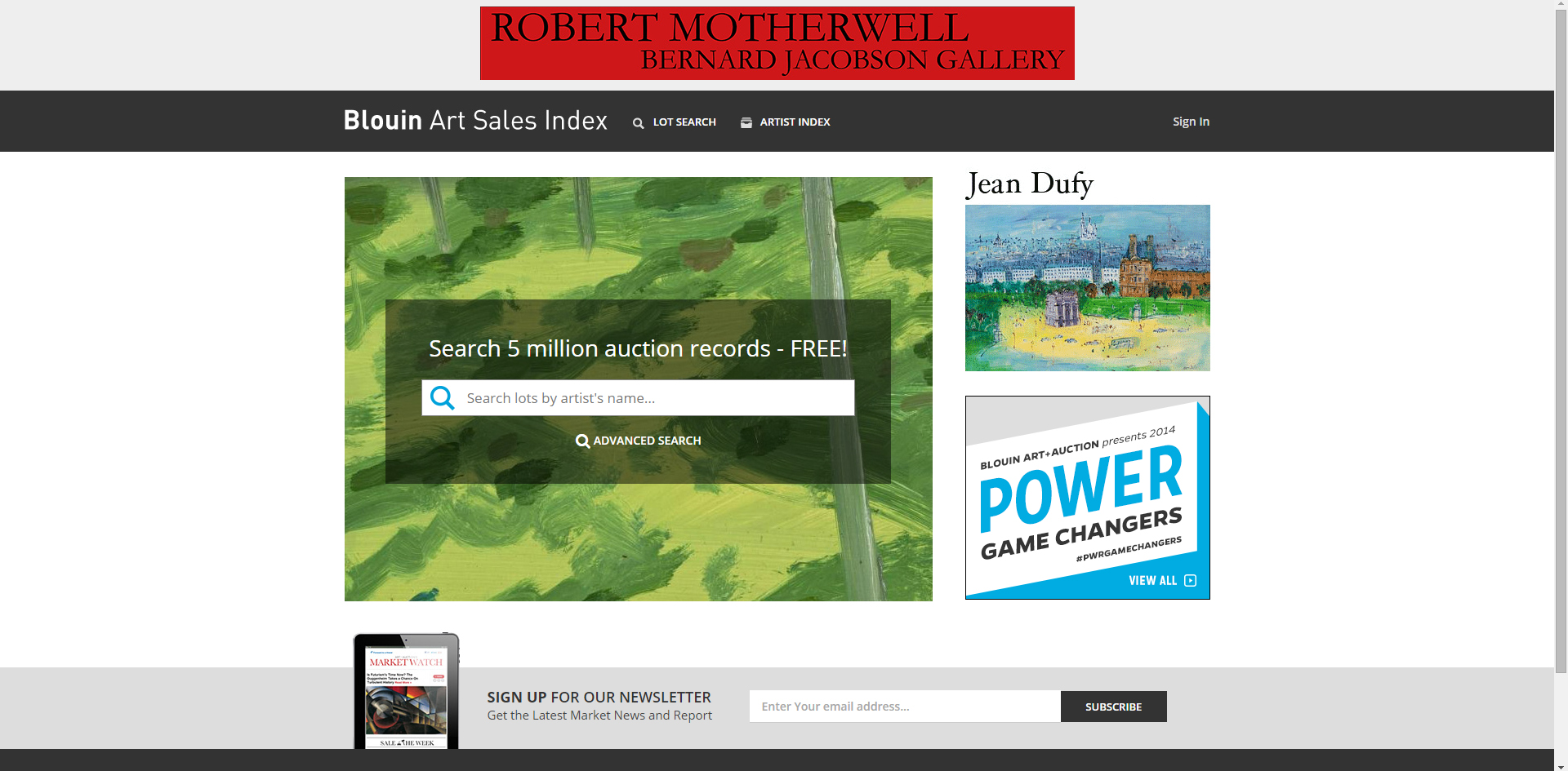
To construct our database for analysis. We looked into the Blouin art sales index website, which has over 5 million auction records for modern paintings.
Part 1 Create Dataframe
To get access to information about each paintings, we actually make a 3-step subsequent query using beautifulsoup
step 1
Using artists' name (alphabet order) - Take 'A' as an example, the url 'http://artsalesindex.artinfo.com/asi/search/artistsAtoZ.ai?lastName=A&startRowNum=' allows access to the artist's paintings. From here we create a list of all url's to their works.
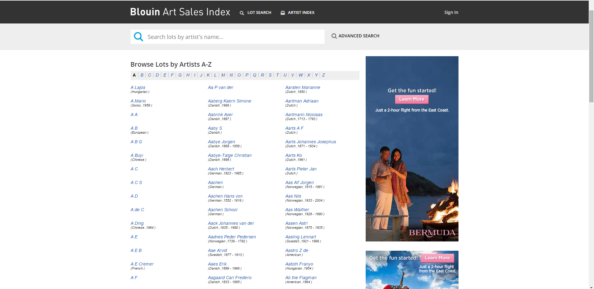
step 2
From each of the url above we come to the booklet of each artists. Here we collect the url's to each individual paintings.
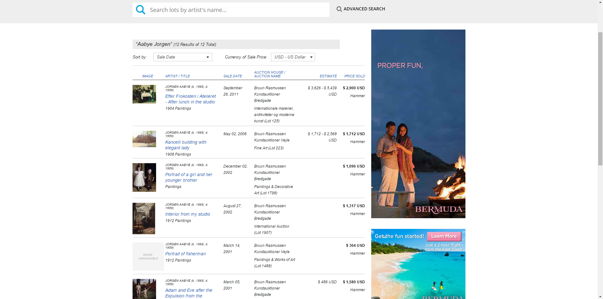
step 3
Finally we have arrive to the info page for each of these artworks. We create our dataframe from these pages.
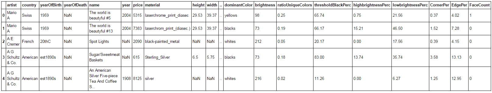
Part 2 Data joining and cleaning
From the dataframe we notice there is some inconsistency and missing fields. Our next step is to join the data set and filter out missing field data. The dataframe looks something like this.
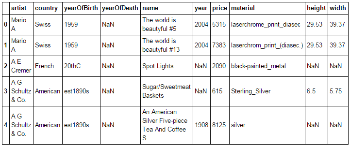
Image processing
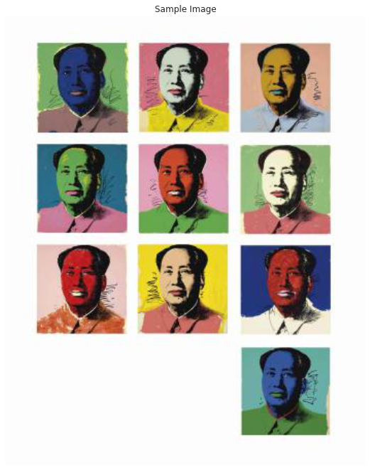
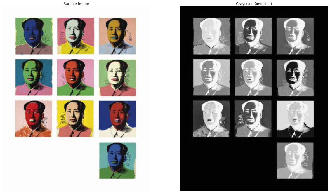
Sample Image
A single image will be used to illustrate the different image processing techniques used in the analysis.
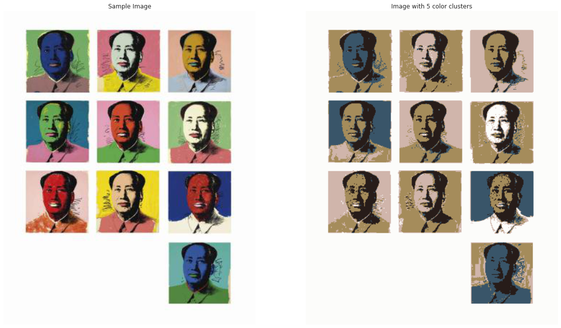
Most Dominant Colors
This function returns the hue of the most dominant color in the image. It first creates a predefined number of clusters from the RGB values in the image array. A larger number of clusters produces a more accurate result but is computationally more expensive. It then assigns codes to each item in the newly clustered array. A histogram counts the number of occurrences of each code. The RGB value that has the highest number of occurrences is the most dominant in the image. A post-processing step is required here. The RGB value of the most dominant color is converted into HSL (hue,saturation, lightness). Thresholding is then used to assign each color to a bucket from the following: blacks, whites, grays, reds, yellows, greens, cyans, blues, magentas, reds
Unique Color Ratio
This function calculates the number of unique colors in an image as a ration of the total number of pixels. A list of color values across the image is generated. Duplicates are removed and the length of the duplicate-free list is calculated and divded by total number of pixels. If the result is close to 0, the image has very few unique colors i.e. large areas of one solid color. If the result is close to 1, the image is very colorful as every pixel has its own unique color. A 0 result indicates a grayscale image.
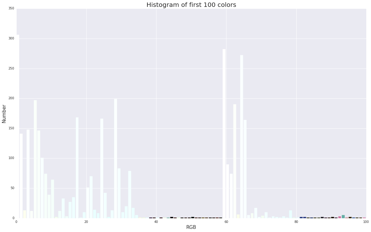
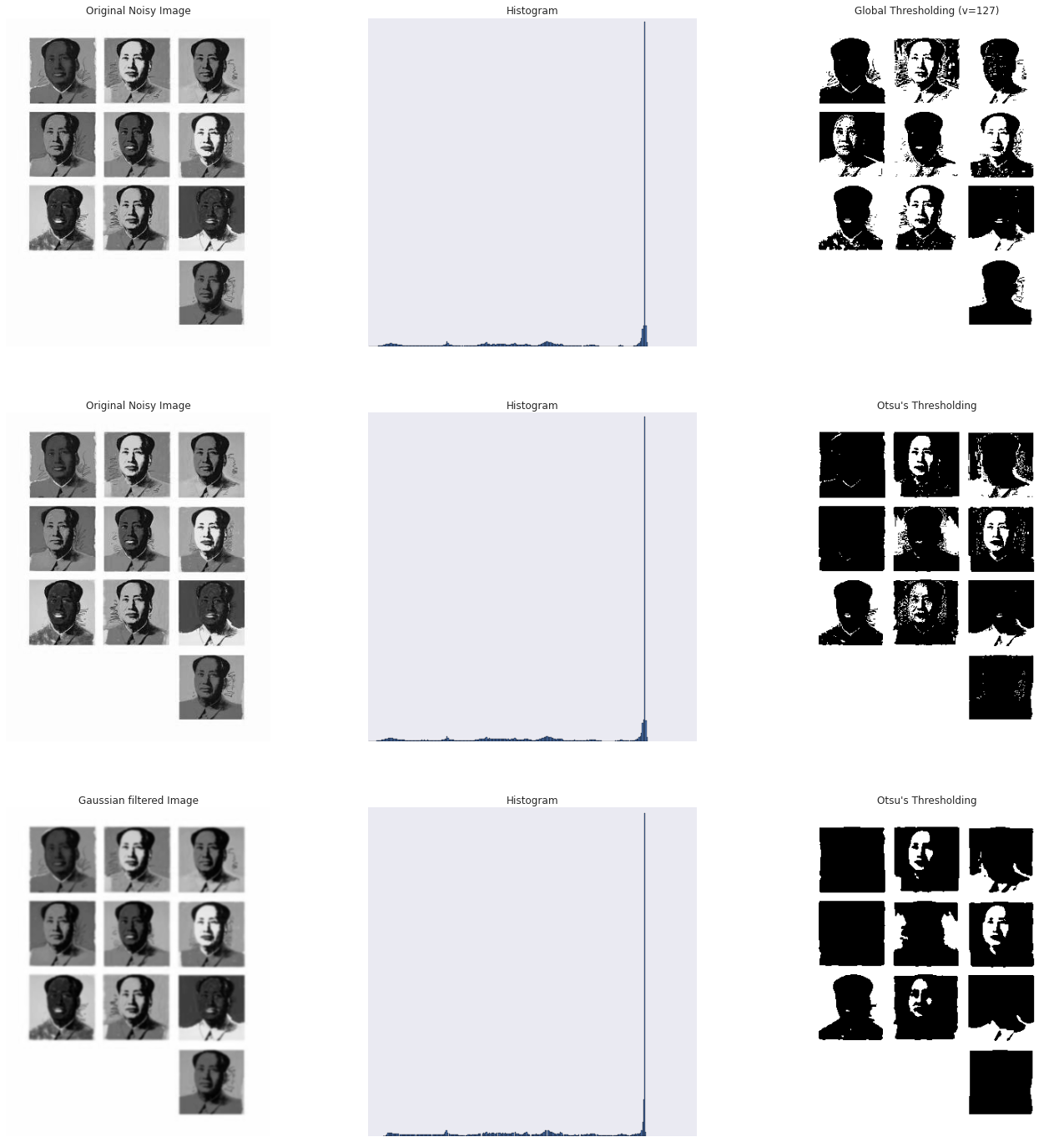
Image Thresholding
Here, we apply a thresholding to the image. If pixel value is greater than a threshold value(here we use 127, range from 0-255), it is assigned one value (255,white), else it is assigned another value (0,black). Then we calculate the Percentage of white or black in the image, so we can get the ratio of black pixels in the greyscale of paintings.
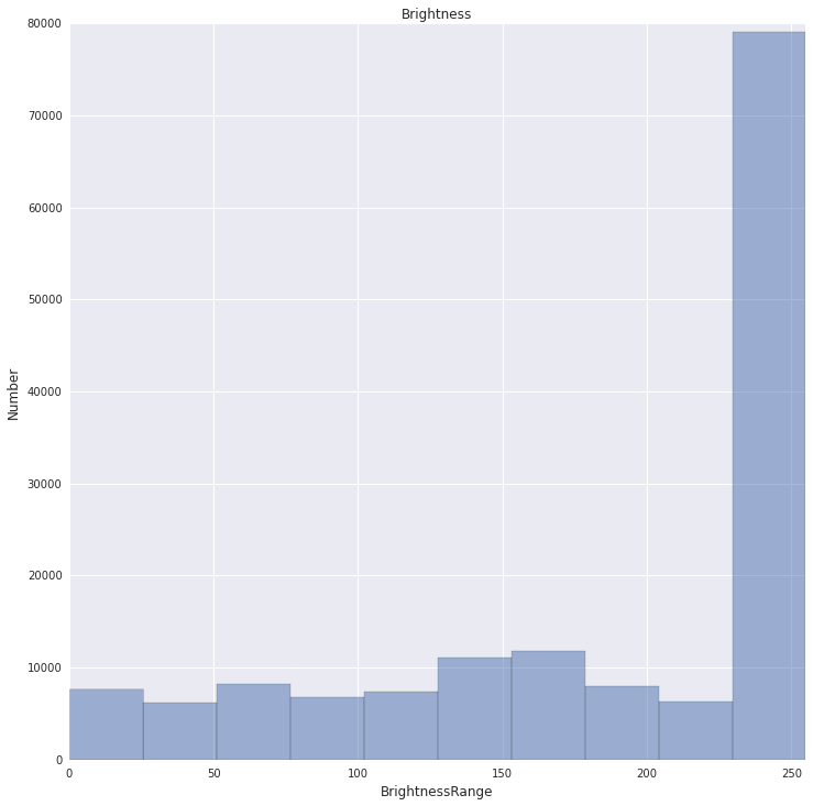
Relative High and low Brightness Ratio
We calculate the average brightness of each paintings here. Then we counts how many pixels have two times of the average brightness and how many pixels have less than half of the mean brightness of that image. So we can get the ratio of these two relatively values of each image. Because different from the mean brightness of overall image, sometimes we say this image has brightness because it has more higher ratio of bright pixels compare to the low pixels. We may get the feeling by comparison. One image has average of 100 brightness but has very low std does not feel more bright than a painting with 90 brightness but has a higher std.
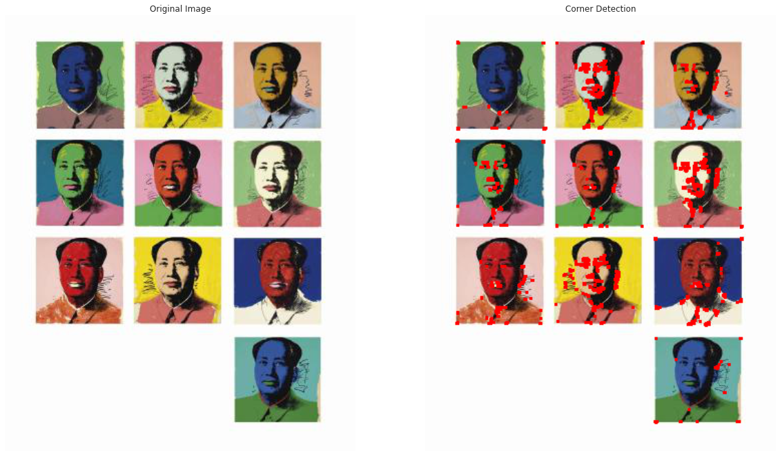
Harris Corner Detection
We use Harris Corner Detection to detect the corner in the paiting. Corner is the intersection of two edges, it represents a point in which the directions of these two edges change. Hence, the gradient of the image (in both directions) have a high variation, which can be used to detect it. With that, we can calcluate the ration of pixels as corners in the full image.
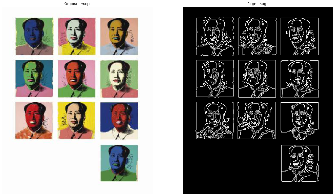
Canny Edge Detection
This function use Canny Edge Detection algorithm to detect the edges in the image. And then calculate the percentage of pixels recognized as edges in the whole picture.
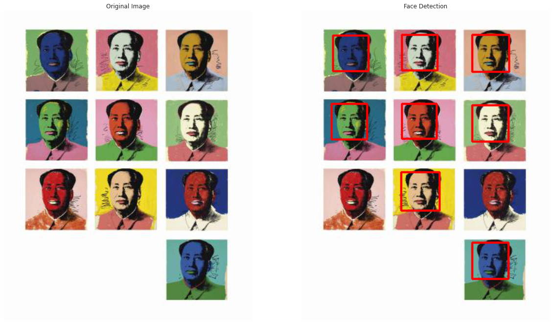
Haar-cascade Face Detection
We use Haar-cascade Detection in OpenCV to detect the face in paintings. With that, we could know whether this looks like a portrait in a way. Because in contemporary paintings, it is hard to understand the image. Portrait does not necessarily means a portrait. We want to test for a paintings which is somewhat readable as human or face will have different influence on the price. We load haarcascade_frontalface_default as XML classifiers. It will show how many faces are detected in the paintings.
Dataframe integration
The output from all these routines is then stored into the previously created dataframe.
"We analyzed 35407 paintings at a total valuation of $9,366,754,845. Prices included a maximum of $119,922,500, an average of $264,545 and a minimum of $3"
Trends
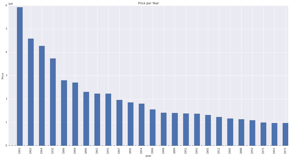
"Paintings produced in the 1960's recorded the highest sales.This coincides with the many artistic impulses that began to gain momentum during that period including the explosion of consumerism and popular culture."
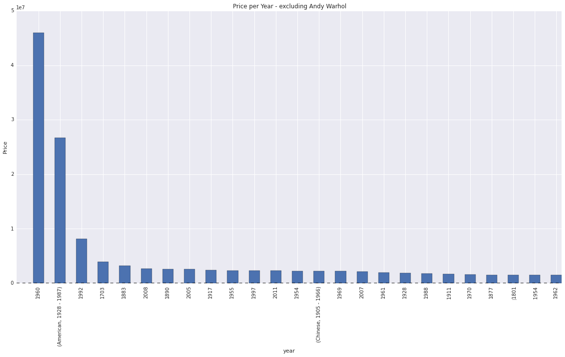
Below is a comparison of prices aggregated per year with and without Andy Warhol.
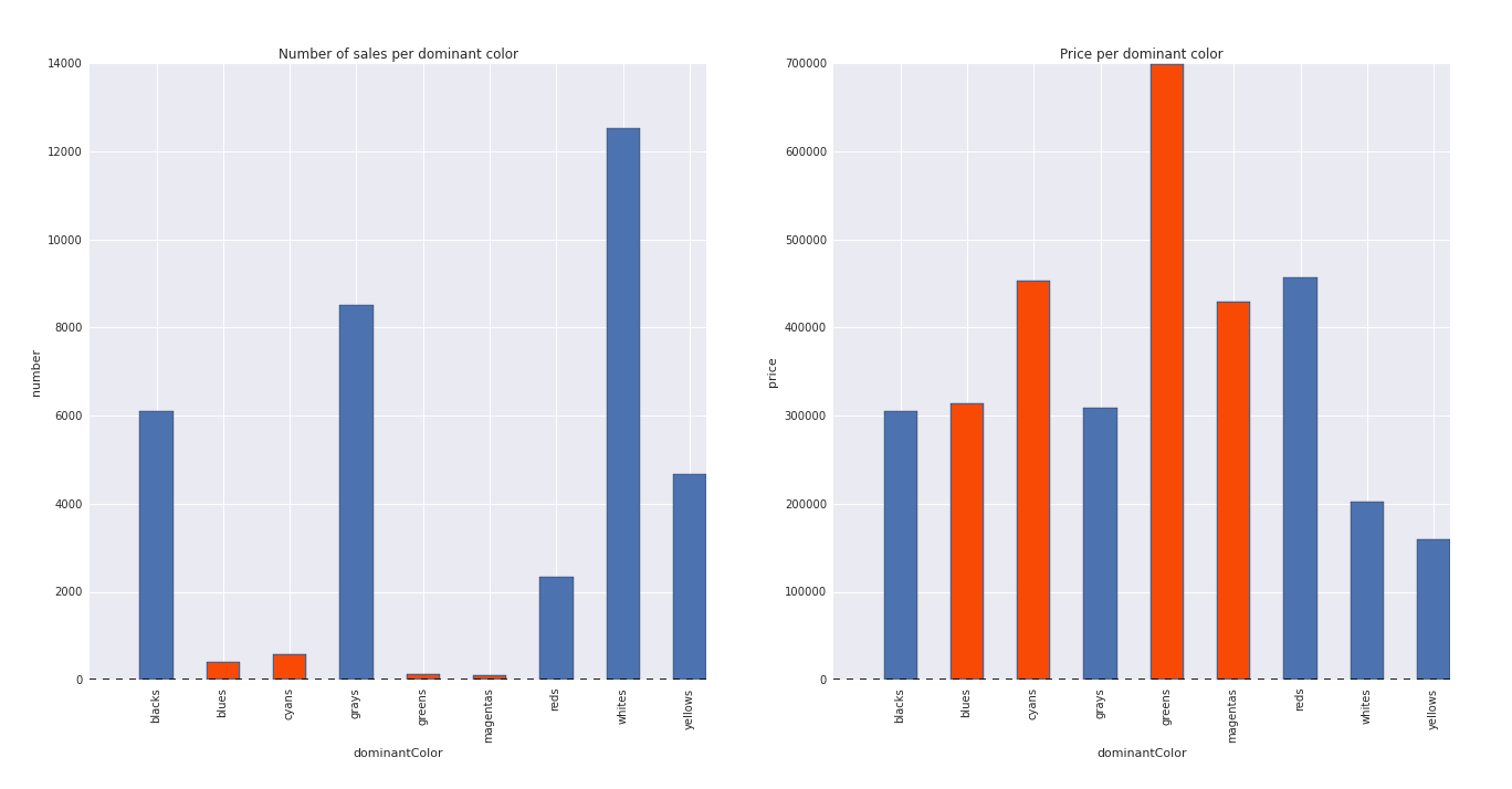
"Paintings with whites, grays and blacks as dominant colors are most likely to have high sales values, compared to other more saturated colors"
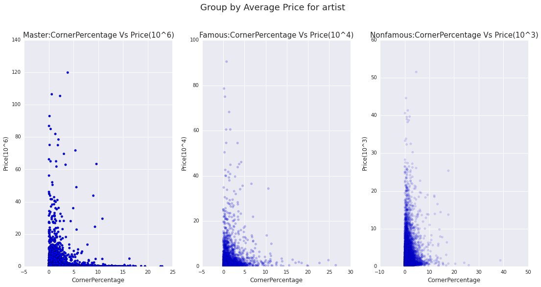
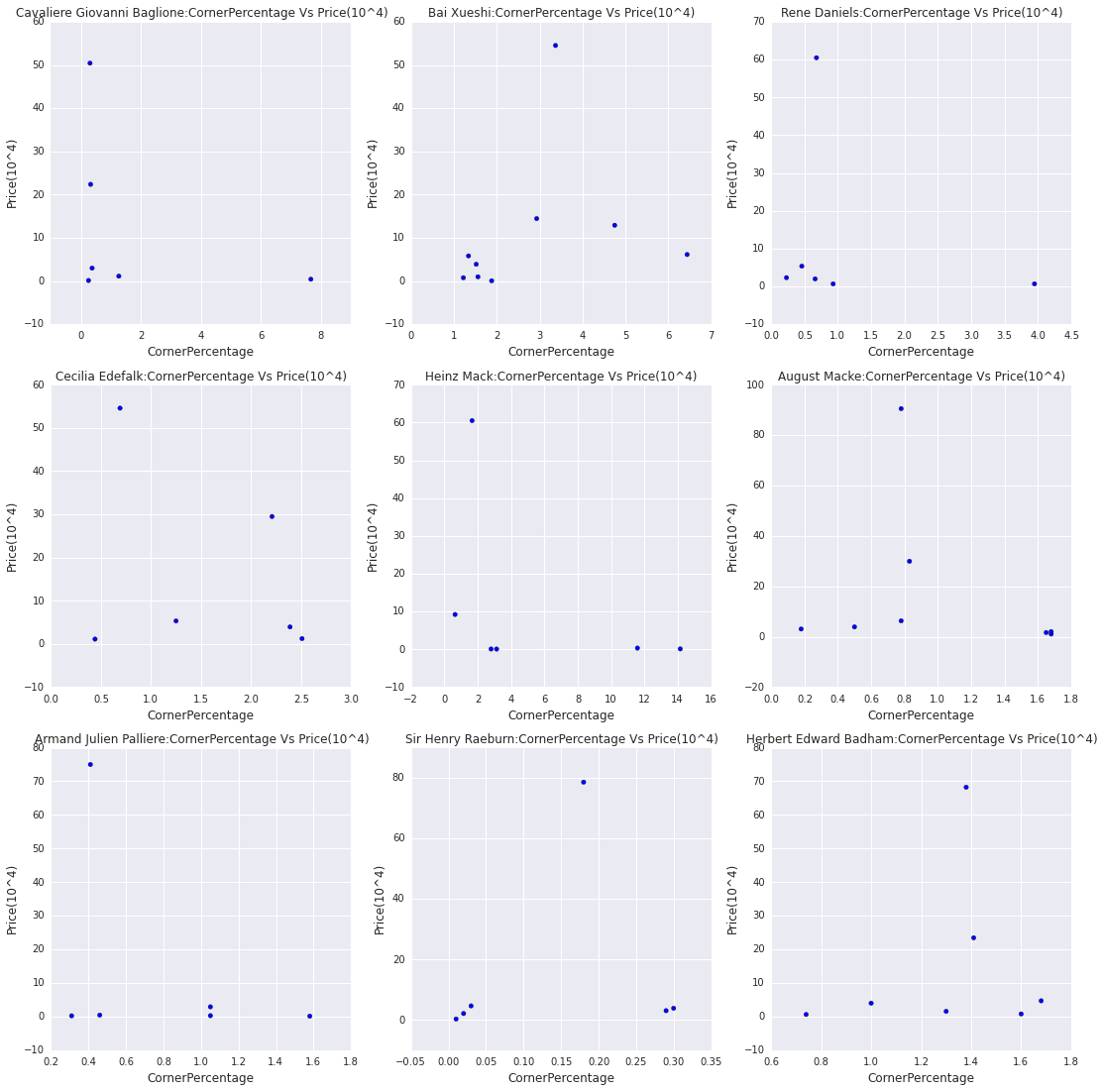
"Paintings where low corner percentages are detected are also more likely to have high sales values."
Below are corner percentages grouped by three artist bands: master, famous and non famous. 9 artists that had large deviation are the plotted separately.
"Auction of very valuable pieces tend to coincide with successful exhibitions."
From these famous artists's principles we've found an interesting feature. They tend to have very high peak at certain time. After research we realize all these moments they have run a very successful exhibition (eg: the Grand Opening of Mark Rothko Art Centre at 2006, Paul Cezanne exhibition 2013 the Museum of Fine Arts in Budapest ...). Then some masterpiece will be on auction. It is very likely that the media advertisement and public exhibition work together to attract attention first, then some really valuable art work will be sold.
.jpg)
.jpg)
Machine Learning
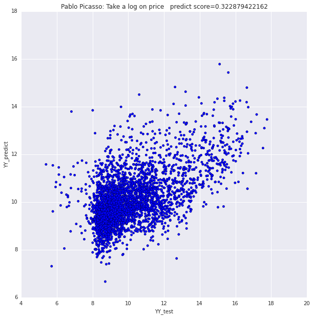
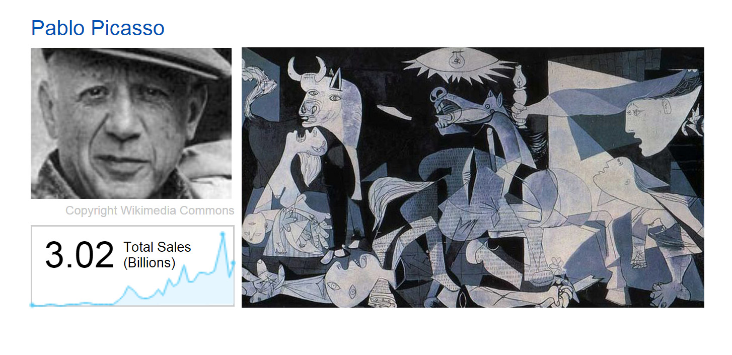
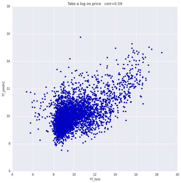
In an attempt to develop a machine learning platform for pricing artwork, we created a linear regression model specifically fit for paintings by Spanish painter Pablo Picasso. We used a set of 4000 paintings for training and another equal set for testing. Our model reached a predicted prices/actual prices correlation of 0.58. Using a single log on the price value gave the most optimum results.
We also built separate regression models based on single parameters as predictors. We noticed that the ratio of unique colors alone generated a relatively high correlation of 0.46 between predicted prices and actual prices.

This allowed us to pick the best performing parametrs for our regression model. The final version of the model scored between 0.32 and 0.34